Disclaimer: This document is not up-to-date. I will eventually write a new post that better reflects the current state of Milton, but in the mean time this is good enough.
After a long time in development, Milton has a brand new renderer. Before now, Milton did all of its rendering on the CPU. The new renderer uses OpenGL to take advantage of the GPU.
I didn’t expect to release OpenGL without problems. I had tested Milton on my machine, which has an Nvidia card. I did some testing with the Intel integrated graphics on this same machine, but I did not do testing with ATI before release.

In the past couple weeks, Milton has gotten some testing from people that aren’t me. At the time of this writing, I am about to ship a new version that corrects some problems with anti-aliasing on non-Nvidia cards.
If Milton works on your machine, then you’ll see how it can handle much more complex paintings now. And for people who use it as a blackboard, which AFAIK is many of Milton’s users thanks to Handmade Hero, it will feel much smoother.
So how does Milton work? Let’s take it step by step.
But first, let me say something!
I tried a million things and failed a million times. This is the second renderer for Milton, and for every part of the new renderer that works there were two or three things that didn’t. Perhaps it would have been better to write a chronological document about the development of the renderer, but it would have been way too long. I am only writing a description of the working result, not the months of work that I spent hitting my head against the wall!
With that said, let us begin.
Creating a new stroke
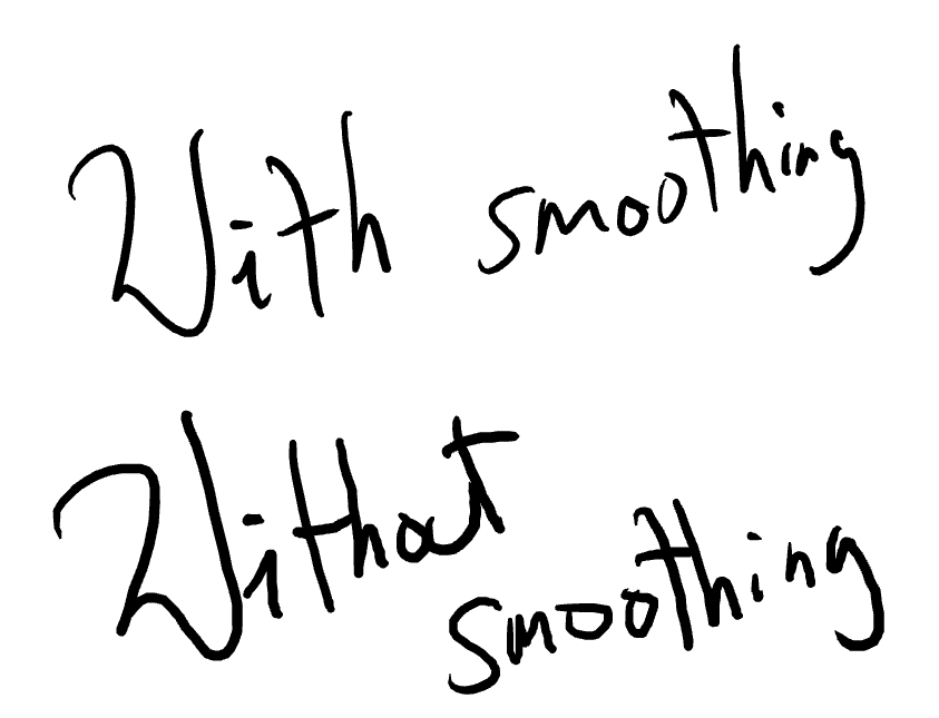
The main loop polls the mouse or (hopefully) the wacom tablet. The mouse gets polled at the Vsync frequency, which is 60hz for most people. This looks really bad. Drawing a circle quickly with the mouse is a great way to create a crappy looking drawing. I will get around to fixing that now that the new renderer is done.
The Wacom is polled at 200hz, or less for lower-end Wacom tablets. The Wacom driver has a limited sample rate. One thing that Milton needs is to do interpolation on the input points.
Milton does some simple smoothing for tablet input. As a stroke is being drawn, every new input point is averaged with the last couple of points. It’s a form of moving average. It’s simple and it works.
Once the stroke is processed, Milton needs to send its information to the GPU, aka “cook it”, so that it can be rendered. A stroke might be cooked several times. If a stroke is within the bounds of the screen and it hasn’t been cooked yet, it gets cooked. If it ever gets within some threshold away from the screen, it gets freed from the GPU.
Canvas space and raster space
Milton works in two different spaces. Raster space is just another name for screen-space coordinates. Canvas space is where Milton strokes live. Every point in raster space is in $[-2^{30}, 2^{30}] \times [-2^{30}, 2^{30}]$.
Milton’s canvas is not really infinite. You can think of it as a $2^{31} \times 2^{31} $ image. A Milton file is a declarative description of a painting in this gigantic canvas, a sort of sparse painting.
Milton interacts with the canvas by mapping the screen rectangle onto a region of the canvas.
We can think of the screen as a window onto the canvas. You can visualize the canvas a very large rectangle, and the screen window as a much smaller rectangle that is always inside. As the user pans, the screen window moves around inside the canvas. When the user zooms out, the window becomes bigger and when they zoom in, it becomes smaller.
Thus, we can speak of a “canvas pixel” in relation to a screen pixel by the following formula:
$$ (x,y)_{canvas} = (x,y)_{screen} * S + P $$
where $S$ is a positive scale value and $P$ is a pan vector.
This means that there fundamental limits to the zoom level. The minimum zoom level is such that every pixel on the screen corresponds to a pixel on the canvas. The maximum possible zoom level is such that the screen window is so large that the whole canvas fits inside it.
In the maximum possible zoom level, the screen window can’t pan anymore because the whole canvas is in view. Milton limits the maximum zoom level so that a user on a 1080p resolution monitor still has about 100 screens of available canvas in every direction.
Milton also limits the minimum zoom, and the reason is that most users like to enlarge their images when exporting. Since the minimum possible zoom corresponds to a 1-to-1 relation between screen pixels and canvas pixels, i.e. $S=1$, the canvas cannot grow bigger because $S$ can’t be smaller. Milton defaults to a minimum value of $S=16$, so that the user can always scale the image up by a reasonable factor when exporting to a bitmap.
Clipping and layers
As a painting gets bigger and bigger, it’s important to do clipping to keep things efficient. This is also important to keep GPU memory usage from growing indefinitely for blackboard-style usage.
Strokes tend to be close together and be of similar size. Milton takes advantage of this with its StrokeList data structure. A StrokeList works like C++ vector. We can append strokes to a StrokeList until we run out of memory. Unlike a C++ vector, but similar to a dequeue implementation, a StrokeList grows by allocating fixed-size buckets, which are fixed-length arrays of strokes with an associated bounding box. A StrokeList is really a linked list of buckets. Every stroke that gets appended to the StrokeList modifies the bounding box of its respective bucket so that it includes the new stroke.
This works well for the intended usage. Large drawings can clip the painting relatively fast by iterating on the buckets and checking the canvas space screen rectangle against the bounding box. The bucket size should be big enough that iteration is fast on modern CPUs but small enough that we get the clustering that we want.
I didn’t try and implement a quadtree or some other spatial subdivision structure. This was the simplest solution that did the job. It is worth noting that before the latest version, Milton did not do any kind of spatial subdivision. I only implemented it after it was clear that it was needed!
Milton has very basic photoshop-style layers. The clipping function leaves data sorted by layer. The bottom layers are rendered first. Within each layer, the oldest strokes are drawn first. Invisible layers simply get clipped out.
Rasterizing strokes
A Milton stroke is an array of points in canvas space. Each point has a corresponding pressure value in $[0,1]$. Every stroke has a color in RGBA, 32-bit floating point per channel.
A stroke is rasterized like this:
for every stroke:
    for every pixel P:
        p = raster_to_canvas(P)  // p is P in canvas space.
        if p is inside stroke:
            blend the stroke
This is not the actual algorithm, but the idea is the same. For instance, Milton does not check every pixel against every stroke, it only checks the pixels that are likely to be shaded by the stroke.
In the interest of space, I won’t go into how the software rasterizer worked. That’s a blog post for another day. Today I will focus on the new renderer.
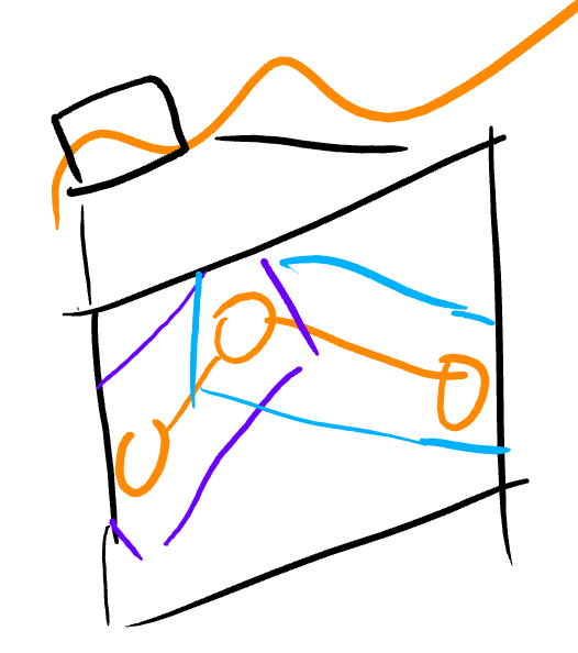
Every stroke (orange) is sent to the GPU in the form of bounding rectangles (purple, blue). Each rectangle represents one segment of the stroke. If a stroke has only one point, the renderer treats it as a segment with two points in the same location.
The rectangles are in canvas space, and they are transformed to raster space in the vertex shader. If we stored strokes in raster space, the whole painting would have to be re-uploaded each time the user panned or zoomed.
Every vertex of the bounding rectangle carries the information two canvas vertices corresponding to a stroke segment - their position and pressure info. This is used in the pixel shader to rasterize the stroke.
Most of the work is done in the pixel shader. The first step is to calculate the closest point in the segment from the canvas space pixel. Just Google for “closest point in segment”. What we are looking for is a value $t \in [0,1]$ such that the point that we are looking for is $a + t(b-a)$, where $a$ and $b$ are the points of the segment. We use $t$ to interpolate the pressure value as well (see the green circles). The pixel is shaded by the stroke if the distance, in canvas space, to the closest point in the segment is less than the brush radius for this stroke times the interpolated pressure value.
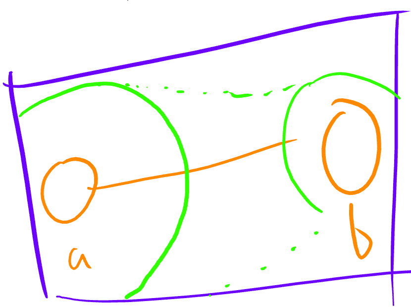
Let’s look at an example to illustrate the rasterization process:

The tricky part about this stroke is the fact that it intersects itself. Milton has to make sure that the pixels at that intersection do not get shaded twice. This important for transparent strokes.
The current solution for this problem is to use the depth buffer, and give each stroke one of $2^{20}$ possible depth values, where the $i$th depth value is $1/i$, for $i \in (0, 2^{20}]$. The depth test is then set to GL_NOT_EQUAL. If there are more than $2^{20}$ strokes in the painting, by the pigeon hole principle there will be two strokes with the same depth value. The algorithm is therefore not correct, but in practice it works. It is much faster than the next best alternative, which was correct, used the stencil buffer and required two draw calls per stroke.
Big shout out to my buddy d7samurai who came up with the depth buffer idea, and also helped me out on twitter with some other OpenGL questions.
Blending
Milton stores colors with premultiplied alpha. This means that if you the color is absolute red rgb = (1,0,0) at 50% opacity, it is stored like this: rgba = (0.5, 0, 0, 0.5).
If we want to blend a color $X = (Xr, Xg, Xb, Xa)$ over another $Y = (Yr, Yg,Yb, Ya)$, the usual formula to use is, for every component $c = r,g,b$, with the color $O$ meaning “X over Y” is $O_c = X_a * X_c + (1 - X_a) * Y_c $
As the name suggests, using premultiplied alpha means that the color value is already multiplied by its alpha, so the over operator looks like $ O_c = X_c + (1-X_a)*Y_c$, which requires one less multiplication.
But the real advantage for Milton is the fact that blending with premultiplied alpha is associative. In other words, if we have three strokes A,B,C, then both ((A over B) over C) and (A over (B over C)) are equivalent. It may help to take a look at an example to see why this matters.
Let’s say we have 100 strokes, S0, S1, ..., S99 covering the area that we want to render. Let’s also say that for some reason, S99, the last stroke (pun not intended), is opaque and completely covering the area (note that the eraser counts as an opaque stroke!). The traditional blending equation would blend (S1 over S0), then it would take that and blend S2 over it, and so on. It would look like ... S4 over (S3 over (S2 over (S1 over S1))). In the end, it would get to S99. Because S99 is opaque, every pixel that was shaded before it is now wasted work. On the other hand, using the associative rule, we could blend in the reverse order. Start with a color that is zero on every component, and blend S99 over it. Then we take that result and blend it over S98. But we can introduce an optimization to avoid that step and finish work for this pixel. We can check that the alpha of the accumulated color is 1.0 and we can avoid the rest of the blend operations!
This was a big deal for the software renderer. It was much less dramatic for the hardware renderer but it was still a win. The current incarnation of the renderer does not have this optimization because of the eraser, but I like this trick so much that I just had to mention it.
Eraser
Eraser strokes work like any other stroke, but while normal strokes get blended as I described, eraser strokes copy texels from an eraser texture onto the final result. The eraser texture starts out being set to the background color, but this is not always the case.
The reason that erasing is hard is layers. Without layers the eraser would simply set pixels to the background color. The problem with layers is that an eraser sets the pixel to whatever is beneath the current layer.
Milton solves the eraser problem by introducing Layer Marks. The main loop of the renderer works by looping over an array of render elements that describe individual strokes. A layer mark is a special kind of render element that is treated differently. When the renderer encounters a layer mark, it takes the current texture (it goes without saying that Milton renders to a texture) and copies it over to the eraser texture. This happens every time there is a new layer to be rendered, which results in the eraser texture always having the contents of whatever is below the current texture.
Anti-Aliasing
Milton uses OpenGL MSAA, but stroke rendering uses an extension called ARB_sample_shading. In traditional OpenGL MSAA, fragments get shaded only once. This usually makes sense for performance, but Milton’s rendering needs every sample to be shaded individually, since the thing that gets aliased is computed in the fragment shader.
The latest bug that I encountered was a problem where ARB_sample_shading behaves different on Nvidia and Intel/AMD. When doing stroke rendering, Nvidia does not need me to specify an offset for the current sample, whereas Intel and AMD do.
Bonus section: Persistent drawing. No save button
After the canvas tech, my favorite Milton feature is the lack of a save button. There is no magic behind this. Milton paintings are very small and computers are very fast.
One argument against this feature is that Milton is written in a language that is not memory safe. If there is a stack stomping bug that corrupts important data, Milton will happily go ahead and save the file for you. I have encountered this problem during development and it could totally happen in the wild. I have AppVerifier turned on for Milton pretty much 100% of the time. I only turn it off when it messes with other tools. AppVerifier has been a huge help to prevent and drastically reduce memory bugs in Milton and my other C/C++ programs. I don’t write Hello World without turning on AppVerifier.
Conclusion
I believe this blog post is a good summary of the interesting parts of Milton. The renderer is the most important part of Milton, but it is only about 10% of the code, not counting third party libraries like dear imgui and SDL.
I always aim to keep things as stupid as possible. I mentioned that Milton didn’t have a spatial subdivision optimization until it was a measurable problem. After it was measurable, I wrote a solution that was tailor-made for Milton and would not work well on other situations. It was a simple solution that solved an actual problem with very little code. I could have started out with a quadtree and ended up with something more complex and less performant.
If I could go back would be to keep things even stupider. The software renderer had many optimizations that made it marginally faster but resulted in code that was harder to understand. By the time I started on the hardware renderer, I had removed most of the smart optimizations in the software renderer. It was mostly a waste of time.
Milton targets OpenGL 3.2 at the moment, but I believe it could lowered to support a bigger set of machines.
I have to stress this again. I tried many different things and rewrote a lot of code before I ended up with the current solution. The first time that the new renderer could show a Milton picture, it took 2 seconds to render a frame, enough to make the driver kill the app. There were many times that I could have thrown my hands and said “fuck it”, and there were a couple of times where I didn’t think that I was going to pull it off. The renderer still has a ways to go, but I am happy and proud of how it has turned out so far.
>> Home